Performance tuning
Performance tuning overview
See also: Case study: Tuning WebSphere Application Server V7 and V8 for performanceTo measure the success of your tests, generate a workload that meets the following characteristics:
| Measurable | Use a metric that can be quantified, such as throughput and response time. |
| Reproducible | Ensure the results can be reproduced when the same test is executed multiple times. Execute tests in the same conditions to define the real impacts of the tuning changes. Change only one parameter at a time. |
| Static | Determine whether the same results can be achieved no matter for how long you execute the run. |
| Representative | Ensure the workload realistically represents the stress to the system under normal operating considerations. Execute tests in a production-like environment with the same infrastructure and the same amount of data. |
Using the queue analogy to tune WebSphere resource pools
WAS functions similarly to a queuing network, with a group of interconnected queues that represent various resources. Resource pools are established for the network, web server, web container, EJB container, ORB, data source, and possibly a connection manager to a custom back-end system. Each of these resources represents a queue of requests waiting to use that resource. Queues are load-dependent resources. As such, the average response time of a request depends on the number of concurrent clients. The tuning of these queues is an essential task to tune for performance.
As an example, think of an application, which consists of servlets and EJB beans, that accesses a database. Each of these application elements reside in the appropriate WebSphere component (for example, servlets in the web container), and each component can handle a certain number of requests in a given time frame.
A client request enters the web server and travels through WebSphere components to provide a response to the client.
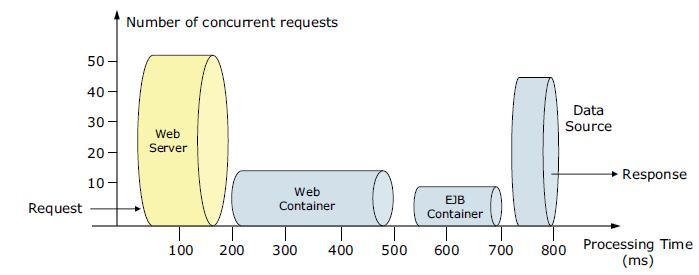
The width of the pipes (illustrated by height) represents the number of requests that can be processed at any given time. The length represents the processing time that it takes to provide a response to the request.
At any given time, a web server can process 50 requests and a web container can process 18 requests. This difference implies that under peak load, requests are queued on the web server side, waiting for the web container to be available. In addition, the EJB container can process nine requests at a given time. Therefore, half of the requests in the web container are also queued, waiting for an ORB thread pool to be available. The database seems to have enough processing power; therefore, requests in the EJB container do not wait for database connections. Suppose that we have adequate CPU and memory in the WAS system. We can increase the ORB pool size to better use the available database connections. Because the web server processes 50 requests at a given time, we can increase the web container thread pool size to more efficiently use the web container threads and to keep up with the increased number of ORB threads. However, how do you determine the maximum amount of threads and database connections? If requests are queued due to processing differences, do you queue them closer to the data layer or closer to the client for best performance? We provide information to help answer these questions in the sections that follow.
Upstream queuing
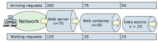
The golden rule of resource pool tuning is to minimize the number of waiting requests in the WAS queues and to adjust resource pools in a way that resources wait in front of the web server. This configuration allows only requests that are ready to be processed to enter the queuing network. To accomplish this configuration, specify the queues furthest upstream (closest to the client) are slightly larger and the queues further downstream (furthest from the client) are progressively smaller. This approach is called upstream queuing.
When 200 client requests arrive at the web server, 125 requests remain queued in the network because the web server is set to handle 75 concurrent clients. As the 75 requests pass from the web server to the web container, 25 requests remain queued in the web server and the remaining 50 requests are handled by the web container. This process progresses through the data source until 25 user requests arrive at the final destination, which is the database server. Because there is work waiting to enter a component at each point upstream, no component in this system must wait for work to arrive. The bulk of the requests wait in the network, outside of WAS. This type of configuration adds stability because no component is overloaded.
Because we do not have an infinite amount of physical resources for the system, do not use equal-sized queues. If we have infinite resources, we can tune the system such that every request from the web server has an available application server thread and every application server thread has an available database connection. However, for most real-world systems, this configuration is not possible.
Another important rule for accurate resource tuning is needed to have a clear understanding of the system infrastructure, application architecture, and requirements. Different systems can have varying access and utilization patterns. For example, in many cases, only a fraction of the requests passing through one queue enters the next queue downstream. However, in a site with many static pages, many requests are fulfilled at the web server and are not passed to the web container.
In this circumstance, the web server queue can be significantly larger than the web container queue. In the previous example, the web server queue was set to 75 requests rather than closer to the value of the Max Application Concurrency parameter. You need to make similar adjustments when different components have different execution times. As the percentage of static content decreases, a significant gap in the web server queue and the application server queue can create poorly performing sites overall.
For another example, in an application that spends 90% of its time in a complex servlet and only 10% of its time making a short JDBC query, on average 10% of the servlets are using database connections at any time. Thus, the database connection pool can be significantly smaller than the web container pool. Conversely, if much of a servlet execution time is spent making a complex query to a database, consider increasing the pool sizes at both the web container and the data source. Always monitor the CPU and memory utilization for both WAS and the database servers to ensure the CPU or memory are not being overutilized.
In the following sections, we provide information about how to tune each resource pool with each pool starting from the furthest downstream, traveling upstream.
Data source tuning
When determining data source queues, consider tuning the following settings:
- Connection pool size
- Prepared statement cache size
Connection pool size
When accessing any database, the initial database connection is an expensive operation. WAS provides support for connection pooling and connection reuse. The connection pool is used for direct JDBC calls within the application and for enterprise beans that use the database.
From IBM Tivoli Performance Viewer go to...
-
JDBC Connection Pools | data source
...and watch...
- Pool Size
- Percent Used
- Concurrent Waiters
Each entity bean transaction requires an additional connection to the database specifically to handle the transaction. Be sure to take this connection into account when calculating the number of data source connections. The connection pool size is set from the dmgr console:
- In the console navigation tree, click...
-
Resources | JDBC Providers | scope (cell, node, or server) | name of the provider | Additional Properties | Data Sources | data source name Connection pool properties
- Use the Minimum connections and Maximum connections fields to configure the pool size.
- Save the configuration, and restart the affected application servers for the changes to take effect.
The default values are 1 for Minimum connections and 10 for Maximum connections. A deadlock can occur if the application requires more than one concurrent connection per thread and if the database connection pool is not large enough for the number of threads. Suppose each of the application threads requires two concurrent database connections and the number of threads is equal to the maximum connection pool size. Deadlock can occur when both of the following statements are true:
- Each thread has its first database connection, and all connections are in use.
- Each thread is waiting for a second database connection, and no connections will become available because all threads are blocked.
To prevent the deadlock in this case, the value set for the database connection pool must be at least one higher than the number of waiting threads to have at least one thread complete its second database connection. To avoid deadlock, code the application to use, at most, one connection per thread. If the application is coded to require concurrent database connections per thread, the connection pool must support at least the following number of connections, where T is the maximum number of threads:
-
T * (C - 1) + 1
The connection pool settings are directly related to the number of connections the database server is configured to support. If you raise the maximum number of connections in the pool and if we do not raise the corresponding settings in the database, the application fails and SQL exception errors are displayed in the SystemErr.log file.
Prepared statement cache size
The data source optimizes the processing of prepared statements to help make SQL statements process faster. It is important to configure the cache size of the data source to gain optimal statement execution efficiency. A prepared statement is a precompiled SQL statement stored in a prepared statement object. This object is used to efficiently execute the given SQL statement multiple times. If the JDBC driver specified in the data source supports precompilation, the creation of the prepared statement sends the statement to the database for precompilation. Some drivers might not support precompilation, and the prepared statement might not be sent until the prepared statement is executed.
If the cache is not large enough, useful entries are discarded to make room for new entries. In general, the more prepared statements the application has, the larger the cache must be. For example, if the application has five SQL statements, set the prepared statement cache size to 5 so that each connection has five statements.
Tivoli Performance Viewer can help tune this setting to minimize cache discards. Use a standard workload that represents a typical number of incoming client requests, a fixed number of iterations, and a standard set of configuration settings. Watch the PrepStmtCacheDiscardCount counter of the JDBC Connection Pools module. The optimal value for the statement cache size is the setting used to get either a value of zero or the lowest value for the PrepStmtCacheDiscardCount counter.
As with the connection pool size, the statement cache size setting requires resources at the database server. Specifying too large a cache can have an impact on database server performance. Consult the database administrator to determine the best setting for the prepared statement cache size.
The statement cache size setting defines the maximum number of prepared statements cached per connection.
We can set the cache size from the dmgr console using these steps:
- In the console navigation tree, select...
-
Resources | JDBC Provider | scope (cell, node or server | provider_name | Additional Properties | Data Sources | data source | WAS data source
- Use the Statement cache size field to configure the total cache size.
- Save the configuration, and restart the affected application servers for the change to take effect.
EJB container
The EJB container can be another source of potential scalability bottlenecks. The inactive pool cleanup interval is a setting that determines how often unused EJB beans are cleaned from memory. Set this interval too low, and the application spends more time instantiating new EJB beans when an existing instance can be reused. Set the interval too high, and the application has a larger memory heap footprint with unused objects that remain in memory. EJB container cache settings can also create performance issues if not properly tuned for the system.
In the sections that follow, we describe the parameters used to make adjustments that might improve performance for the EJB container.
Cache settings
To determine the cache absolute limit, multiply the number of enterprise beans that are active in any given transaction by the total number of concurrent transactions expected. Next, add the number of active session bean instances. Use Tivoli Performance Viewer to view bean performance information.
The cache settings consist of the following parameters:
- The cache size: The cache size specifies the number of buckets in the active instance list within the EJB container.
- The cleanup interval: The cleanup interval specifies the interval at which the container attempts to remove unused items from the cache to reduce the total number of items to the value of the cache size.
To change these settings, click...
-
Servers | Application servers AppServer_Name | EJB Container Settings | EJB container | EJB cache settings
The default values are Cache size=2053 buckets and Cache cleanup interval=3000 milliseconds.
ORB thread pool size
Method invocations to enterprise beans are only queued for requests coming from remote clients going through the RMI activity service. An example of such a client is an EJB client running in a separate JVM (another address space) from the enterprise bean. In contrast, no queuing occurs if the EJB client (either a servlet or another enterprise bean) is installed in the same JVM the EJB method runs on and the same thread of execution as the EJB client.
Remote enterprise beans communicate using the RMI/IIOP protocol. Method invocations initiated over RMI/IIOP are processed by a server-side ORB. The thread pool acts as a queue for incoming requests. However, if a remote method request is issued and there are no more available threads in the thread pool, a new thread is created. After the method request completes, the thread is destroyed. Therefore, when the ORB is used to process remote method requests, the EJB container is an open queue because of the use of unbounded threads.
Tivoli Performance Viewer can help tune the ORB thread pool size settings. Use a standard workload that represents a typical number of incoming client requests, a fixed number of iterations, and a standard set of configuration settings. Watch the PercentMaxed counter of the Thread Pools module. If the value of this counter is consistently in the double digits, the ORB might be a bottleneck, and we need to increase the number of threads in the pool.
The degree to which we need to increase the ORB thread pool value is a function of the number of simultaneous servlets (, clients) that are calling enterprise beans and the duration of each method call. If the method calls are longer or if the applications spend a lot of time in the ORB, consider making the ORB thread pool size equal to the web container size. If the servlet makes only short-lived or quick calls to the ORB, servlets can potentially reuse the same ORB thread. In this case, the ORB thread pool can be small, perhaps even one-half of the thread pool size setting of the web container.
We can configure the ORB thread pool size from the dmgr console by completing the following steps:
- To change these settings, click EJB cache settings.
- Click...
-
Servers | Application servers | appserver | Container Services | ORB Service | Thread Pool
- Use the Maximum Size field to configure the maximum pool size. Note that this setting affects only the number of threads that are held in the pool. The actual number of ORB threads can be higher.
- Save the configuration, and restart the affected application server for the change to take effect.
Web container tuning
Monitor the web container thread pool closely during initial performance runs. This bottleneck is the most common bottleneck in an application environment. Define the web container size, considering all the infrastructure chain in close cooperation with the web server number of threads and the number of sessions of the database. If you adjust the number of threads to be too low, the web server threads can wait for the web container. If you adjust the number of threads to be too high, the back end can be inundated with too many requests. For both circumstances, the consequence is an increase of the response time or even a hang.To route servlet requests from the web server to the web containers, a transport connection between the web server plug-in and each web container is established. The web container manages these connections through transport channels and assigns each request to a thread from the web container thread pool.
Web container thread pool
The web container maintains a thread pool to process inbound requests for resources in the container (servlets and JSP pages). To monitor, use a standard workload representing a typical number of incoming client requests, a fixed number of iterations, and a standard set of configuration settings, then from the Thread Pools module, watch...
- PercentMaxed
- ActiveCount
If the value of the PercentMaxed counter is consistently in the double digits, the web container can be a bottleneck, and we need to increase the number of threads. Alternatively, if the number of active threads are significantly lower than the number of threads in the pool, consider lowering the thread pool size for a performance gain.
To set web container thread pool size...
-
Servers | Application servers | AppServer_Name | Additional Properties | Thread Pools | WebContainer | Maximum Size
Note that in contrast to the ORB, the web container uses threads only from the pool. Thus, this configuration is a closed queue. Default is 50.
Save the configuration, and restart the affected application server for the change to take effect.
To allow for an automatic increase of the number of threads beyond the maximum size configured for the thread pool.
-
Allow thread allocation beyond maximum thread size
Selecting this can lead to the system becoming overloaded.
HTTP transport channel maximum persistent requests
Maximum persistent requests is the maximum number of requests allowed on a single keep-alive connection. This parameter can help prevent denial of service attacks when a client tries to hold on to a keep-alive connection. The web server plug-in keeps connections open to the application server as long as it can, providing optimum performance. A good starting value for the maximum number of requests allowed is 100 (which is the default value). If the application server requests are received from the web server plug-in only, increase this value.
To configure the maximum number of requests allowed...
-
Servers | Application servers | AppServer | Container Settings | Web Container Settings | Web container transport chains | transport chain | HTTP Inbound Channel (HTTP #) | Maximum persistent requests
Save the configuration, and restart the affected application server for the change to take effect.
Web server tuning - concurrent requests
The web server must allow for sufficient concurrent requests to make full use of the application server infrastructure. The web server also acts as a filter and keeps users waiting in the network to avoid flooding the servers if more requests than the system can handle are incoming. As a rough initial start value for testing the maximum concurrent threads (one thread can handle one request at a time), use the following setting:
-
MaxClients = (((TH + MC) * WAS) * 1.26) / WEB
...where...
| TH | Number of threads in the web container |
| MC | MaxConnections setting in the plugin-cfg.xml |
| WAS | Number of WAS servers |
| WEB | Number of web servers |
If we are using IBM HTTP Server, server-status will show the number of web server threads going to the web container, and the number of threads accessing static content locally on the web server. For additional information about IHS performance tuning...
- Tuning IBM HTTP Server to maximize the number of client connections to WebSphere Application Server
- IBM HTTP Server Performance Tuning
A simple way to determine the correct queue size for any component is to perform a number of load runs against the application server environment at a time when the queues are large, ensuring maximum concurrency through the system. For example, one approach might be as follows:
- Set the queue sizes for the web server, web container, and data source to initial values.
Set the values to estimate initial values for the web container and ORB thread pools.
- Simulate a large number of typical user interactions entered by concurrent users in an attempt to fully load the WebSphere environment.
In this context, concurrent users means simultaneously active users that send a request, wait for the response, and immediately re-send a new request upon response reception. We can use any stress tool to simulate this workload, such as IBM Rational Performance Tester.
- Measure overall throughput, and determine at what point the system capabilities are fully stressed (the saturation point).
- Repeat the process, each time increasing the user load. After each run, record the throughput (requests per second) and response times (seconds per request), and plot the throughput curve.
The throughput of WAS is a function of the number of concurrent requests that are present in the total system. At some load point, congestion develops due to a bottleneck and throughput increases at a much lower rate until reaching a saturation point (maximum throughput value). The throughput curve can help you identify this load point.
It is desirable to reach the saturation point by driving CPU utilization close to 100% because this point gives an indication that a bottleneck is not caused by something in the application. If the saturation point occurs before system utilization reaches 100%, it is likely that another bottleneck is being aggravated by the application. For example, the application might be creating Java objects that are causing excessive garbage collection mark phase bottlenecks in Java. You might notice these bottlenecks because only one processor is being used at a time on multi-processor systems. On uniprocessor systems, you will not notice the symptom but will notice only the problems the symptom causes.
Throughput curve...

Section A contains a range of users that represent a light user load. The curve in this section illustrates that as the number of concurrent user requests increase, the throughput increases almost linearly with the number of requests. We can interpret this increase to mean that at light loads, concurrent requests face little congestion within the WAS system queues.
In the heavy load zone, Section B, as the concurrent client load increases, throughput remains relatively constant. However, the response time increases proportionally to the user load. That is, if the user load is doubled in the heavy load zone, the response time doubles.
In Section C (the buckle zone), one or more of the system components became exhausted and throughput degrades. For example, the system might enter the buckle zone if the network connections at the web server exhaust the limits of the network adapter or if the requests exceed operating system limits for file handles.
Estimating web container and ORB thread pool initial sizes
Tuning WebSphere thread pools is a critical activity that has impact on the response time of the applications that run on WebSphere. Although allocating less than an optimum number of threads can result in higher response times, allocating higher then the optimum number can result in over use of system resources, such as CPU, databases, and other resources. A load test can determine the optimum number for thread pool sizes.When tuning for performance, we are most frequently tuning web container thread and ORB thread pools. As a starting point, we need to know the possible use cases of the applications and the kind of workload generated by these use cases. Suppose that we have an online banking application. One use case for a user is to log in, check account details, transfer money to another account, and then log out. You need to estimate how many web and EJB requests are generated by each activity in this use case. (You might also want to gather statistics about how many data source connections this use case uses and for how long it uses these connections.) Next, we need to calculate an estimate of requests for all use cases and determine the total requests per second for the system.
Suppose the application receives 50 HTTP requests and 30 EJB requests per second.
The expected average response time for web requests is 1 second and for EJB requests the response time is 3 seconds. In this case, we need the following minimum number of threads:
- Web Container Thread Pool: 50/1= 50
- EJB Container Thread Pool: 30/3 = 10
Maximum number of threads that we need depends on the difference between the load in peak time and the average load. Suppose that we have 1.5 times the average load in peak time. Then, we need the following maximum number of threads:
- Web Container Thread Pool = 50 x 1.5 = 75
- EJB Container Thread Pool = 10 x 1.5 = 15
WebSphere Plug-in tuning
In the Web server plug-in, the following parameters can be tuned to obtain the best performance:
- LoadBalanceWeight
Is a starting "weight". The value is dynamically changed by the Plug-in during runtime. The "weight" of a server (or clone) is lowered each time a request is assigned to that clone.
When all weights for all servers drop to 0 or below, the Plug-in has to readjust all of the weights so they are above 0. The usual configuration for LoadBalanceWeight is to set all application servers with the same value, except one, which is configured with a value off by one (for example: 20, 20, 19).
- MaxConnections
This parameter is used to determine when a server is "starting to become overwhelmed" but not to determine when to fail-over (mark a server "down").
When a request is sent to an active server, the request is PENDING until handled by the back-end application server. Requests that are handled quickly, will only be PENDING for a short time. Therefore, under ideal conditions, the MaxConnections setting should be set to its default value (-1). However, when application servers are pushed handling a large volume of requests and the handling of incoming requests is taking more time to complete, PENDING requests start to build up. In these cases, the parameter MaxConnections can be used to put a limit on the number of PENDING requests per server. When this limit is met, the server is unavailable for additional new requests but is not marked down.
The optimal value for MaxConnections depends on how quickly the application and to run these two phases. By default, the number of threads used is limited by the number of CPUs. Compaction occurs if required. As the name implies, this policy favors a higher throughput than the other policies. Therefore, this policy is more suitable for systems that run batch jobs. However, because it does not include concurrent garbage collection phases, the pause times can be longer than the other policies.
The optavgpause policy
This policy uses concurrent garbage collection to reduce pause times. Concurrent garbage collection reduces the pause time by performing some garbage collection activities concurrently with normal program execution. This method minimizes the disruption caused by the collection of the heap. This policy limits the effect of increasing the heap size on the length of the garbage collection pause. Therefore, it is most useful for configurations that have large heaps. This policy provides reduced pause times by sacrificing throughput.
The gencon policy
This policy is the default garbage collection policy for WAS V8.5, and it is the short name for concurrent garbage collection and generational garbage collection combined. This policy includes both approaches to minimize pause times. The idea behind generational garbage collection is splitting the Java heap into two areas, nursery and tenured. New objects are created in a nursery area and, if they continue to be reachable for the tenure age (a defined number of garbage collections), they are moved into the tenured area.
This policy dictates a more frequent garbage collection of only the nursery area rather than collecting the whole heap as the other policies do. The local garbage collection of the nursery area is called scavenge. The gencon policy also includes a concurrent mark phase (not a concurrent sweep phase) for the tenured space, which decreases the pause times of a global garbage collection.The gencon policy can provide shorter pause times and more throughput for applications that have many short-lived objects. It is also an efficient policy against heap fragmentation problems because of its generational strategy.
The balanced policy
We can use the balanced policy only on 64-bit platforms that have compressed references enabled. This policy involves splitting the Java heap into equal sized areas called regions. Each region can be collected independently, allowing the collector to focus on the regions that return the largest amount of memory for the least processing effort. Objects are allocated into a set of empty regions that are selected by the collector. This area is known as an eden space.
When the eden space is full, the collector stops the application to perform a partial garbage collection. The collection might also include regions other than the eden space, if the collector determines these regions are worth collecting. When the collection is complete, the application threads can proceed, allocating from a new eden space, until this area is full. Balanced garbage collection incrementally reduces fragmentation in the heap by compacting part of the heap in every collection. By proactively tackling the fragmentation problem in incremental steps, the balanced policy eliminates the accumulation of work sometimes incurred by generational garbage collection, resulting in less pause times.
From time to time, the collector starts a global mark phase to detect if there are any abandoned objects in the heap that are unrecognized by previous partial garbage collections. During these operations, the JVM attempts to use under utilized processor cores to perform some of this work concurrently while the application is running. This behavior reduces any stop-the-world time the operation might require.
The subpool policy
The subpool policy works on SMP systems (AIX, Linux PPC, and IBM eServer zSeries, and z/OS and i5/OS� only) with 16 or more processors. This policy aims to improve performance of object allocations using multiple free lists called subpools rather than the single free list used by the optavgpause and optthruput policies. Subpools have varying sizes. When allocating objects on the heap, a subpool with a "best fit" size is chosen, as opposed to the "first fit" method used in other algorithms. This policy also tries to minimize the amount of time for which a lock is held on the Java heap. This policy does not use concurrent marking. The subpool policy provides additional throughput optimization on the supported systems.
Comparison of garbage collection policies
Summarizes characteristics and results for different garbage collection policies. Note that some of the results, such as yielding to higher throughput times, is common to more than one policy because all policies that have this result achieve it using different algorithms. If your aim is to have higher throughput for the system, you might want to test with all the policies that have this result, as listed in Table 15-1, and come up with the best policy for the system.Comparison of garbage collection policies
| Policy name | Results |
|---|---|
| Optthruputt | Higher throughput, longer response times for applications with GUI |
| Optavgpause | Less pause times, shorter response times for applications with GUI. Shorter pause times for large heaps |
| Gencon | High throughput when application allocates short-lived objects. Shorter response times due to local garbage collection. Effective against heap fragmentation |
| Balanced | Reduces pause times by incremental compactions. Uses NUMA hardware for higher performance. Dynamically unload unused classes and class loaders on every partial collect. Uses under used cores for the global mark phase |
| Subpool | Additional throughput optimization on the supported systems |
Sizing the JVM heap
We can set minimum and maximum heap sizes that are equal, instead of setting a minimum heap size smaller than the maximum heap size. This approach prevents heap expansions and compactions that might occur if the minimum heap size is set smaller than the maximum heap size. However, this approach can have the following drawbacks:
- Because the minimum heap size is larger, it takes more time for the collections.
- Because many compactions are omitted, this approach can lead to a more fragmented heap than the minimum less than maximum approach, especially if we are not using generational garbage collection policies.
To set initial and maximum heap sizes...
- Servers | Application servers | server_name | System Infrastructure | Java and Process Management | Process definition | JVM
Set the initial heap value in the Initial heap size field. Set the maximum heap value in the Maximum heap size field.
Save the configurations to the master repository, synchronize the nodes, and recycle the application server that was reconfigured.
We can also use the following JVM arguments to set the minimum and maximum heap sizes:
-
-Xms<size> Sets the initial Java heap size.
-Xmx<size> Sets the maximum Java heap size.
In a load tests, the best approach is to first set the minimum and maximum values to be equal and then determine the optimum heap size for the system by trying different sizes. After you find the optimum number, set the minimum and maximum values around this number, and then test to find the best performing minimum and maximum values. We can compare performance with these different values to see which settings are optimal for the system.
Avoid setting low values for the initial heap size, especially when the maximum heap is configured to high values. Example: When we have a maximum heap size of 1536MB, do not set the initial heap size value to 50MB (default value for the initial heap size) because this causes performance degradation due to an excessive load on the garbage collector. As a general rule, setting the initial heap size to at least 50% of the maximum heap can be a good starting point to determine the optimum values for the environment.
Sizing the nursery and tenured space when using the gencon policy
The duration of the nursery collect is determined by the amount of data copied from the allocate space to the survivor space, which are two different regions in the nursery space. The size of the nursery does not have an increasing effect on scavenges. Instead, increasing the nursery size increases the time between scavenges, which decreases the amount of data copied.
The amount of live data that can be copied to the nursery at any time is limited by the amount of transactions that can work concurrently, which is fixed by the container pool settings. Thus, the nursery size can be fixed to an optimum large value. By default, the nursery size is a quarter of the total heap size or 64 MB, whichever is smaller. The nursery can shrink and expand within this size.
We can use the following parameters to define the nursery size:
| -Xmns<size> | Initial size of the new (nursery) area. Default is 25% of the value of -Xms. |
| -Xmnx<size> | Maximum size of the new (nursery) area. Default is 25% of the value of -Xmx. |
| -Xmn<size> | Initial and maximum size of the new (nursery) area. Equivalent to setting both -Xmns and -Xmnx. |
We can use the following parameters to define the tenured space size:
| -Xmos<size> | Initial size of the old (tenure) heap. Default is 75% of the value of -Xms. |
| -Xmox<size> | Maximum size of the old (tenure) heap. Default is same value as -Xmx. |
| -Xmo<size> | Initial and maximum size of the old (tenured) heap. Equivalent to setting both -Xmos and -Xmox. |
For a starting point, we can use -Xmn to fix the size of the nursery space to a large enough value. Then, we can treat the tenured space as a Java heap with a non-generational policy, and use the -Xmos and -Xmox parameters to replace -Xms and -Xmx.
Use compressed references
The IBM SDK for Java 64-bit stores object references as 64-bit values. The -Xcompressedrefs command-line option causes object references to be stored as 32-bit representations, which reduces the 64-bit object size to be the same as a 32-bit object. Because the 64-bit objects with compressed references are smaller than default 64-bit objects, they occupy a smaller memory footprint in the Java heap and improve data locality. Generally, this parameter results in better memory utilization and improved performance. We can perform load testing and compare the results to see whether using this parameter improves performance for the application.
-
Servers | Server Types | WebSphere application servers | server_name | Java and process management | ProcessDefinition | Environment entries
Select a scope based on your desired affected environment.
In the name field, click New, and specify IBM_JAVA_OPTIONS. In the Value field, add or append the -Xcompressedrefs.
Synchronize changes and restart servers.
Other tuning considerations
This section describes other tuning considerations that can help and guide you when tuning for performance.
Dynamic caching
The dynamic cache service improves performance by caching the output of servlets, commands, and JavaServer Pages (JSP) files. WAS consolidates several caching activities, including servlets, web services, and WebSphere commands, into one service called the dynamic cache. These caching activities work together to improve application performance and share many configuration parameters that are set in an application server's dynamic cache service.
The dynamic cache works within an application server JVM, intercepting calls to cacheable objects, for example, through a servlet's service() method or a command's execute() method. The dynamic cache either stores the object's output to or serves the object's content from the dynamic cache. Because J2EE applications have high read/write ratios and can tolerate small degrees of latency in the currency of their data, the dynamic cache can create an opportunity for significant gains in server response time, throughput, and scalability.
The pass by reference parameter
Passing EJB beans by value can be expensive in terms of resource use because of the forever remote method call. The parameters are copied onto the stack before the call is made.We can use the pass by reference parameter, which passes the original object reference without making a copy of the object, to avoid this impact.
For EJB 2 or later and 3 or later beans, interfaces can be local or remote. For local interfaces, method calls use the pass by reference parameter by default. If the EJB client and EJB server are installed in the same WAS instance and if the client and server use remote interfaces, specifying the pass by reference parameter can improve performance up to 50%. Note that using the pass by reference parameters helps performance only when non-primitive object types are being passed as parameters. Therefore, int and floats are always copied, regardless of the call model. Also, be aware that using the pass by reference parameter can lead to unexpected results. If an object reference is modified by the remote method, the change might be seen by the caller. As a general rule, any application code that passes an object reference as a parameter to an enterprise bean method or to an EJB home method must be scrutinized to determine if passing that object reference results in loss of data integrity or in other problems.
To set this value, use the dmgr console to complete the following steps:
- Click...
-
Servers | Application servers | <AppServer_Name> | Container Services | ORB Service
- Select the Pass by reference parameter.
- Click OK and then click Apply to save the changes.
- Stop and restart the application server.
Large page support
Many operating systems provide the ability to use a larger memory page size than the default memory page size of 4 KB. Having larger page sizes decreases CPU consumption because the CPU has to manage fewer pages. Therefore, Java applications often benefit from using large pages.To enable large page utilization, configure the value on your operating system.
Application tuning
The most important part of your tuning activities is spent on the application. The majority of performance-related problems are related to application design and development implementations. Only a well-designed application, developed with the preferred practices for programming, can give you good throughput and response times. Although environment-related tuning is important to optimize resource use and to avoid bottlenecks, it cannot compensate for a poorly written application.
Review the application code itself as part of the regular application life cycle to ensure that it is using the most efficient algorithms and the most current APIs available for external dependencies. For example, take care to use optimized database queries or prepared statements instead of dynamic SQL statements. To help you in this task, we can optimize the application performance using application profiling.
Tools
This section provides information about the tools that can help and guide you when tuning for performance.
Tivoli Performance Viewer
Tivoli Performance Viewer is included with WAS V8.5 and is used to record and display performance data. Using Tivoli Performance Viewer, we can perform the following tasks:- Display PMI data collected from local and remote application servers
Summary reports show key areas of contention. It also provides graphical and tabular views of raw PMI data.
- Provide configuration advice through the performance advisor section
We can formulate tuning advice from gathered PMI and configuration data.
- Log performance data
Using Tivoli Performance Viewer, we can log real-time performance data and review the data at a later time.
- View server performance logs
We can record and view data logged using Tivoli Performance Viewer in the Integrated Solutions Console.
Collect Java dumps and core files
With WAS V8.5, we can produce a Java dump, Java core, or system dump files directly using the dmgr console. These files are useful when we have performance issues needed to analyze, such as memory, thread, and system behaviors.
To collect Java dump and core files:
- Click Troubleshooting | Java dumps and cores.
- Select the server or servers.
- Click System Dump, Java Core, or Heap Dump, as appropriate.
IBM Pattern Modelling and Analysis Tool for Java Garbage Collector
IBM Pattern Modelling and Analysis Tool for Java Garbage Collector (PMAT) analyzes verbose garbage page trace. It provides crucial information for garbage collection tuning, such as verbose garbage collection analysis, verbose garbage collection graphics, list of errors, and recommendations.We can enable verbose garbage page by selecting the option in the JVM Settings window
IBM Monitoring and Diagnostic tools for Java
IBM Monitoring and Diagnostic tools for Java are available using IBM Support Assistant, which is a workbench that offers a single point to access these tools. Using IBM Monitoring and Diagnostic tools for Java, we can analyze applications, garbage collection files, Java heap dump files, and Java core files.| Health center | Monitor the real-time running applications and provides useful information about memory, class loading, I/Os, object allocations, and the system. This tool can help you to identify application memory leaks, I/O bottlenecks, and lock contentions and can help you to tune the garbage collector. The health center is designed to minimize the performance impact of the monitoring. |
| Memory analyzer | Analyze the Java heap of a JVM process, identifies potential memory leaks, and provides the application memory footprint. Memory analyzer provides a useful object tree browsing function to focus on the objects interactions and to analyze the memory usage. |
| Dump analyzer | Determine the causes of Java crashes by analyzing the operating system dump. This analysis can be useful to better understand the application failures. |
| Garbage collection and memory visualizer | Analyze and tune the garbage collection, similar to PMAT. It also provides recommendations to optimize the garbage collector and to find the best Java heap settings. Garbage collection and memory visualizer allow you to browse the garbage collection cycles and to better understand the memory behavior of the application. |
IBM HTTP server status monitoring page
To monitor IBM HTTP Server, a useful web page called server-status is available. This page is disabled by default, but we can enable it in the httpd.conf configuration file. This web page displays a real-time view of the current IBM HTTP Server state, which includes the following information:
- The CPU usage
- The total number of requests served since the server is up
- The total traffic size since the server is up
- Some average about the response time
- The number of requests currently running
- The number of idle threads
- And the list of the requests being processed
To enable the server status monitoring page:
- Edit the IBM HTTP Server httpd.conf file, and remove the comment character (#) from the following lines in this file:
#LoadModule status_module, modules/ApacheModuleStatus.dll,
#<Location/server-status>
#SetHandler server-status
#</Location>
- Save the changes, and restart IBM HTTP Server.
- In a web browser, go to: http://your_host/server-status. Click Reload to update the status. If the browser supports refresh, go to
-
http://your_host/server-status?refresh=5
...to refresh every 5 seconds.
WebSphere performance advisors
When gathering runtime information, the WebSphere performance advisors provide diagnostic advice about the environment. The advisors can determine the current configuration for an application server. Then, by trending the runtime data over time, the advisors provide advice about potential environmental changes that can enhance the performance of the system. The advice is hard coded into the system and is based on IBM preferred practices for tuning and performance.
The advisors do not implement any changes to the environment. Instead, they identify the problem and allow the system administrator to make the decision as to whether to implement. Perform tests after any change is implemented.
WebSphere provides the following types of advisors:
- Performance and Diagnostic Advisor
- Performance Advisor in Tivoli Performance Viewer
Performance and Diagnostic Advisor
This advisor is configured through the Integrated Solutions Console. It writes to the application server log files and to the console while in monitor mode. To minimize the performance impact, configure the server to use HPEL instead of using the systemOut.log file.
The interface is configurable to determine how often data is gathered and how often advice is written. It offers advice about the following components:
- J2C Connection Manager:
- Thread pools
- LTC Nesting
- Serial reuse violation
- Plus various different diagnostic advises
- Web Container Session Manager:
- Session size with overflow enabled
- Session size with overflow disabled
- Persistent session size
- Web Container:
- Bounded thread pool
- Unbounded thread pool
- Orb Service:
- Unbounded thread pool
- Bounded thread pool
- Data Source:
- Java JVM:
- Memory leak detection
If we need to gather advice about items that are outside of this list, use the Performance Advisor in Tivoli Performance Viewer.
The Performance Advisor in Tivoli Performance Viewer
This advisor is slightly different from the Performance and Diagnostic Advisor. The Performance Advisor in Tivoli Performance Viewer is invoked only through the Tivoli Performance Viewer interface of the Integrated Solutions Console. It runs on the application server that we are monitoring, but the refresh intervals are based on selecting refresh through the console. Also, the output is routed to the user interface instead of to an application server output log file. This advisor captures data and gives advice about more components. Specifically, this advisor can capture the following types of information:
- ORB service thread pools
- Web container thread pools
- Connection pool size
- Persisted session size and time
- Prepared statement cache size
- Session cache size
- Dynamic cache size
- JVM heap size
- DB2 performance configuration
Running the Performance Advisor in Tivoli Performance Viewer requires resources and can impact performance. Use it with care in production environments.
Case Study
A complete performance tuning case study for WAS
The case study describes how different configurations behave, does a comparison between the different settings, and shows how to extract valuable data from the tests. This information can help you apply the optimum configuration values into application servers settings.