Planning your worker node setup
Red Hat OpenShift on IBM Cloud provides different worker node flavors and isolation levels so that you can choose the flavor and isolation that best meet the requirements of the workloads that we want to run in the cloud.
A worker node flavor describes the compute resources, such as CPU, memory, and disk capacity that you get when you provision the worker node. Worker nodes of the same flavor are grouped in worker node pools. The total number of worker nodes in a cluster determine the compute capacity that is available to your apps in the cluster.
Trying to plan how many worker nodes your need in your cluster? Check out Sizing your Kubernetes cluster to support the workload to find information about the default worker node setup and how you can determine the resource requirements of the workloads.
Available hardware for worker nodes
The worker node flavors and isolation levels that are available to you depend on your container platform, cluster type, the infrastructure provider that we want to use, and the Red Hat OpenShift on IBM Cloud location where we want to create your cluster.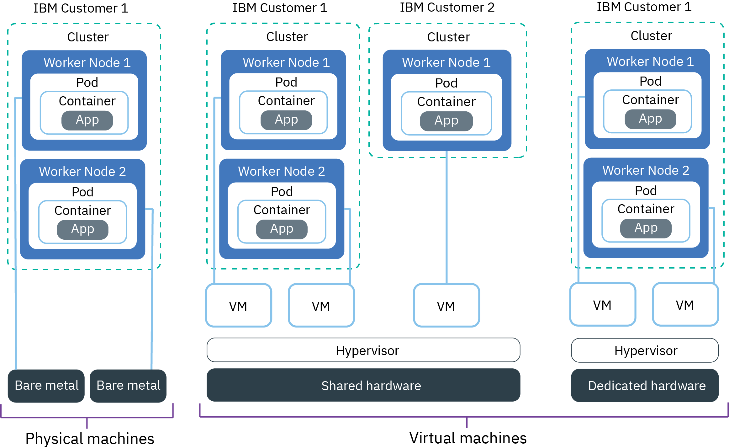
What flavors are available to me?
Classic standard clusters can be created on virtual and bare metal worker nodes. If you require additional local disks, you can also choose one of the
bare metal flavors that are designed for software-defined storage solutions, such as Portworx. Depending on the level of hardware isolation that we need, virtual worker nodes can be set up as shared or dedicated nodes,
whereas bare metal machines are always set up as dedicated nodes. If you create a free classic cluster, your cluster is provisioned with the smallest virtual worker node flavor on shared infrastructure.
VPC clusters can be provisioned as standard clusters on shared virtual worker nodes only, and must be created in one of the supported multizone-capable metro cities. Free VPC clusters are not supported.
Can I combine different flavors in a cluster?
Yes. To add different flavors to your cluster, we must create another worker pool.
You cannot resize existing worker pools to have different compute resources such as CPU or memory.
How can I change worker node flavors?
See updating flavors.
Are the worker nodes encrypted?
The secondary disk of the worker node is encrypted. For more information, see Overview of cluster encryption. After you
create a worker pool, we might notice that the worker node flavor has .encrypted in the name, such as b3c.4x16.encrypted.
How do I manage my worker nodes?
Worker nodes in classic clusters are provisioned into your IBM Cloud account. You can manage your worker nodes by using Red Hat OpenShift on IBM Cloud, but you can also use the classic infrastructure dashboard in the IBM Cloud console to work with your worker node directly.
Unlike classic clusters, the worker nodes of your VPC cluster are not listed in the VPC infrastructure dashboard. Instead, you manage your worker nodes with Red Hat OpenShift on IBM Cloud only. However, your worker nodes might be connected to other VPC infrastructure resources, such as VPC subnets or VPC Block Storage. These resources are included in the VPC infrastructure dashboard and can be managed separately from there.
What limitations do I need to be aware of?
Kubernetes limits the maximum number of worker nodes that you can have in a cluster. Review worker node and pod quotas for more information.
Reserved capacity and reserved instances are not supported.
Why do my worker nodes have the master role?
When you run oc get nodes or oc describe node <worker_node>, we might see that the worker nodes have master,worker roles. In OpenShift clusters, operators use the master role as a nodeSelector so that the operators can deploy properly to your worker nodes. No master node processes occur on the worker nodes.
Red Hat OpenShift on IBM Cloud also sets compute resource reserves that limit available compute resources on each worker node. For more information, see worker node resource reserves.
Want to be sure that you always have enough worker nodes to cover the workload? Try out the cluster autoscaler.
Virtual machines
With VMs, you get greater flexibility, quicker provisioning times, and more automatic scalability features than bare metal, at a more cost-effective price. You can use VMs for most general-purpose use cases such as testing and development environments, staging, and prod environments, microservices, and business apps. However, there is a trade-off in performance. For high-performance computing for data- or RAM-intensive workloads, consider creating classic clusters with bare metal worker nodes.Planning considerations for VMs
Do I want to use shared or dedicated hardware?
When you create a standard classic cluster, we must choose whether we want the underlying hardware to be shared by multiple IBM customers (multi tenancy) or to be dedicated
to you only (single tenancy). VPC standard clusters can be provisioned on shared infrastructure (multi tenancy) only.
To achieve HIPAA and PCI compliance for your environment, make sure to use dedicated virtual or bare metal machines for your worker nodes, not shared virtual machines. With dedicated virtual or bare metal machines, all compute resources are dedicated exclusively to you, and you can control the isolation and resource consumption of the workloads.
- In a multi-tenant, shared hardware setup: Physical resources, such as CPU and memory, are shared across all virtual machines that are deployed to the same physical hardware. To ensure that every virtual machine can run independently, a virtual machine monitor, also referred to as the hypervisor, segments the physical resources into isolated entities and allocates them as dedicated resources to a virtual machine (hypervisor isolation).
- In a single-tenant, dedicated hardware setup: All physical resources are dedicated to you only. You can deploy multiple worker nodes as virtual machines on the same physical host. Similar to the multi-tenant setup, the hypervisor assures that every worker node gets its share of the available physical resources.
Shared nodes are usually less costly than dedicated nodes because the costs for the underlying hardware are shared among multiple customers. However, when you decide between shared and dedicated nodes, we might want to check with your legal department to discuss the level of infrastructure isolation and compliance that your app environment requires.
Some classic worker node flavors are available for only one type of tenancy setup. For example, m3c VMs can be provisioned in a shared tenancy setup only. Additionally, VPC clusters are available as only shared virtual machines.
How does storage work for VMs?
Every VM comes with an attached disk for storage of information that the VM needs to run, such as OS file system, container runtime, and the kubelet. Local storage on the worker
node is for short-term processing only, and the storage disks are wiped when you delete, reload, replace, or update the worker node. For persistent storage solutions for your apps, see Planning highly available persistent storage.
Additionally, classic and VPC infrastructure differ in the disk setup.
 Classic VMs: Classic VMs have two attached disks. The primary storage disk has 25 GB for the
OS file system, and the secondary storage disk has 100 GB for data such as the container runtime and the kubelet. For reliability, the primary and secondary storage volumes are local disks instead of storage area networking
(SAN). Reliability benefits include higher throughput when serializing bytes to the local disk and reduced file system degradation due to network failures. The secondary disk is encrypted by default.
Classic VMs: Classic VMs have two attached disks. The primary storage disk has 25 GB for the
OS file system, and the secondary storage disk has 100 GB for data such as the container runtime and the kubelet. For reliability, the primary and secondary storage volumes are local disks instead of storage area networking
(SAN). Reliability benefits include higher throughput when serializing bytes to the local disk and reduced file system degradation due to network failures. The secondary disk is encrypted by default.
 VPC compute VMs: VPC VMs have one primary disk that is a block storage volume that is attached via
the network. The storage layer is not separated from the other networking layers, and both network and storage traffic are routed on the same network. To account for network latency, the storage disks have a maximum of up to 3000 IOPS.
The primary storage disk is used for storing data such as the OS file system, container runtime, and kubelet, and is encrypted by default.
VPC compute VMs: VPC VMs have one primary disk that is a block storage volume that is attached via
the network. The storage layer is not separated from the other networking layers, and both network and storage traffic are routed on the same network. To account for network latency, the storage disks have a maximum of up to 3000 IOPS.
The primary storage disk is used for storing data such as the OS file system, container runtime, and kubelet, and is encrypted by default.
Available flavors for VMs
The following table shows available worker node flavors for classic and VPC clusters. Worker node flavors vary by cluster type, the zone where we want to create the cluster, the container platform, and the infrastructure provider that you want to use. To see the flavors available in your zone, run ibmcloud oc flavors --zone <zone>.
If your classic cluster has deprecated x1c or older Ubuntu 16 x2c worker node flavors, you can update your cluster to have Ubuntu 18 x3c worker nodes.
Classic clustersVPC Gen 2 computeScroll for moreScroll for more| Name and use case | Cores/ Memory | Primary/ Secondary disk | Network speed |
|---|---|---|---|
| Virtual, b3c.4x16: Select this balanced VM for testing and development, and other light workloads. | 4 / 16 GB | 25 GB / 100 GB | 1000 Mbps |
| Virtual, b3c.16x64: Select this balanced VM for mid-sized workloads. | 16 / 64 GB | 25 GB / 100 GB | 1000 Mbps |
| Virtual, b3c.32x128: Select this balanced VM for mid to large workloads, such as a database and a dynamic website with many concurrent users. | 32 / 128 GB | 25 GB / 100 GB | 1000 Mbps |
| Virtual, c3c.16x16: Use this flavor when we want an even balance of compute resources from the worker node for light workloads. | 16 / 16 GB | 25 GB / 100 GB | 1000 Mbps |
| Virtual, c3c.16x32: Use this flavor when we want a 1:2 ratio of CPU and memory resources from the worker node for light to mid-sized workloads. | 16 / 32 GB | 25 GB / 100 GB | 1000 Mbps |
| Virtual, c3c.32x32: Use this flavor when we want an even balance of compute resources from the worker node for mid-sized workloads. | 32 / 32 GB | 25 GB / 100 GB | 1000 Mbps |
| Virtual, c3c.32x64: Use this flavor when we want a 1:2 ratio of CPU and memory resources from the worker node for mid-sized workloads. | 32 / 64 GB | 25 GB / 100 GB | 1000 Mbps |
| Virtual, m3c.4x32: Use this flavor when we want a 1:8 ratio of CPU and memory resources for light workloads that require more memory, similar to databases such as Db2 on Cloud. Available only in Dallas and as --hardware shared tenancy. | 4 / 32 GB | 25 GB / 100 GB | 1000 Mbps |
| Virtual, m3c.8x64: Use this flavor when we want a 1:8 ratio of CPU and memory resources for light to mid-sized workloads that require more memory, similar to databases such as Db2 on Cloud. Available only in Dallas and as --hardware shared tenancy. | 8 / 64 GB | 25 GB / 100 GB | 1000 Mbps |
| Virtual, m3c.16x128: Use this flavor when we want a 1:8 ratio of CPU and memory resources for mid-sized workloads that require more memory, similar to databases such as Db2 on Cloud. Available only in Dallas and as --hardware shared tenancy. | 16 / 128 GB | 25 GB / 100 GB | 1000 Mbps |
| Virtual, m3c.30x240: Use this flavor when we want a 1:8 ratio of CPU and memory resources for mid to large-sized workloads that require more memory, similar to databases such as Db2 on Cloud. Available only in Dallas and as --hardware shared tenancy. | 30 / 240 GB | 25 GB / 100 GB | 1000 Mbps |
| Virtual, z1.2x4: se this flavor when we want a worker node to be created on Hyper Protect Containers on IBM Z Systems. | 2 / 4 GB | 25 GB / 100 GB | 1000 Mbps |
| Name and use case | Cores / Memory | Primary disk | Network speed * |
|---|---|---|---|
| Virtual, b1.8x32: Select this balanced VM if we want a 1:4 ratio of CPU and memory resources from the worker node for light to mid-sized workloads. | 8 / 32 GB | 100 GB | 1000 Mbps |
| Virtual, b2.4x16: Select this balanced VM if we want a 1:4 ratio of CPU and memory resources from the worker node for testing, development, and other light workloads. | 4 / 16 GB | 100 GB | 1000 Mbps |
| Virtual, b2.8x32: Select this balanced VM if we want a 1:4 ratio of CPU and memory resources from the worker node for light to mid-sized workloads. | 8 / 32 GB | 100 GB | 1000 Mbps |
| Virtual, b2.16x64: Select this balanced VM if we want a 1:4 ratio of CPU and memory resources from the worker node for mid-sized workloads. | 16 / 64 GB | 100 GB | 1000 Mbps |
| Virtual, b2.32x128: Select this balanced VM if we want a 1:4 ratio of CPU and memory resources from the worker node for large-sized workloads. | 32 / 128 GB | 100 GB | 1000 Mbps |
| Virtual, b2.48x192: Select this balanced VM if we want a 1:4 ratio of CPU and memory resources from the worker node for large-sized workloads. | 48 / 192 GB | 100 GB | 1000 Mbps |
| Virtual, c2.4x8: Use this flavor when we want a 1:2 ratio of CPU and memory resources from the worker node for light-sized workloads. | 4 / 8 GB | 100 GB | 1000 Mbps |
| Virtual, c2.8x16: Use this flavor when we want a 1:2 ratio of CPU and memory resources from the worker node for light to mid-sized workloads. | 8 / 16 GB | 100 GB | 1000 Mbps |
| Virtual, c2.16x32: Use this flavor when we want a 1:2 ratio of CPU and memory resources from the worker node for mid-sized workloads. | 16 / 32 GB | 100 GB | 1000 Mbps |
| Virtual, c2.32x64: Use this flavor when we want a 1:2 ratio of CPU and memory resources from the worker node for mid to large-sized workloads. | 32 / 64 GB | 100 GB | 1000 Mbps |
| Virtual, m2.4x32: Use this flavor when we want a 1:8 ratio of CPU and memory resources from the worker node for light to mid-sized workloads that require more memory. | 4 / 32 GB | 100 GB | 1000 Mbps |
| Virtual, m2.8x64: Use this flavor when we want a 1:8 ratio of CPU and memory resources from the worker node for mid-sized workloads that require more memory. | 8 / 64 GB | 100 GB | 1000 Mbps |
| Virtual, m2.16x128: Use this flavor when we want a 1:8 ratio of CPU and memory resources from the worker node for mid to large-sized workloads that require more memory. | 16 / 128 GB | 100 GB | 1000 Mbps |
| Virtual, m2.32x256: Use this flavor when we want a 1:8 ratio of CPU and memory resources from the worker node for large-sized workloads that require more memory. | 32 / 256 GB | 100 GB | 1000 Mbps |
* VPC Gen 2: For more information about network performance caps for virtual machines, see VPC Gen 2 compute profiles. The network speeds refer to the speeds of the worker node interfaces. The maximum speed available to your worker nodes is 16Gbps. Because IP in IP encapsulation is required for traffic between pods that are on different VPC Gen 2 worker nodes, data transfer speeds between pods on different worker nodes might be slower, about half the compute profile network speed. Overall network speeds for apps that we deploy to your cluster depend on the worker node size and application's architecture.
Physical machines (bare metal)
You can provision the worker node as a single-tenant physical server, also referred to as bare metal.![]() Physical machines are available for classic clusters only and are not supported in VPC clusters.
Physical machines are available for classic clusters only and are not supported in VPC clusters.
Planning considerations for bare metal
How is bare metal different than VMs?
Bare metal gives you direct access to the physical resources on the machine, such as the memory or CPU. This setup eliminates the virtual machine hypervisor that allocates physical
resources to virtual machines that run on the host. Instead, all of a bare metal machine's resources are dedicated exclusively to the worker, so you don't need to worry about "noisy neighbors" sharing resources or slowing
down performance. Physical flavors have more local storage than virtual, and some have RAID to increase data availability. Local storage on the worker node is for short-term processing only, and the primary and secondary disks are wiped
when you update or reload the worker node. For persistent storage solutions, see Planning highly available persistent storage.
Because we have full control over the isolation and resource consumption for the workloads, you can use bare metal machines to achieve HIPAA and PCI compliance for your environment.
Besides better specs for performance, can I do something with bare metal that I can't with VMs?
Yes, with bare metal worker nodes, you can use IBM Cloud Data Shield. IBM Cloud Data Shield is integrated with
Intel® Software Guard Extensions (SGX) and Fortanix® technology so that your IBM Cloud container workload code and data are protected in use. The app code and data run in CPU-hardened enclaves. CPU-hardened enclaves are trusted areas of
memory on the worker node that protect critical aspects of the app, which helps to keep the code and data confidential and unmodified. If you or your company require data sensitivity due to internal policies, government regulations, or industry
compliance requirements, this solution might help you to move to the cloud. Example use cases include financial and healthcare institutions, or countries with government policies that require on-premises cloud solutions.
For supported flavors, see the IBM Cloud Data Shield documentation.
Bare metal sounds awesome! What's stopping me from ordering one right now?
Bare metal servers are more expensive than virtual servers, and are best suited for high-performance apps that need more resources and host
control. Bare metal worker nodes are also not available for VPC clusters.
Bare metal servers are billed monthly. If you cancel a bare metal server before the end of the month, we are charged through the end of that month. After you order or cancel a bare metal server, the process is completed manually in your IBM Cloud infrastructure account. Therefore, it can take more than one business day to complete.
Available flavors for bare metal
Worker node flavors vary by cluster type, the zone where we want to create the cluster, the container platform, and the infrastructure provider that we want to use. To see the flavors available in your zone, run ibmcloud oc flavors --zone <zone>. You can also review available VM or SDS flavors.
Bare metal machines are optimized for different use cases such as data- or RAM-intensive workloads. GPU bare metal machines are not available for Red Hat OpenShift on IBM Cloud clusters, but you can order GPU bare metal for IBM Cloud Kubernetes Service clusters.
Choose a flavor, or machine type, with the right storage configuration to support the workload. Some flavors have a mix of the following disks and storage configurations. For example, some flavors might have a SATA primary disk with a raw SSD secondary disk.
- SATA: A magnetic spinning disk storage device that is often used for the primary disk of the worker node that stores the OS file system.
- SSD: A solid-state drive storage device for high-performance data.
- Raw: The storage device is unformatted and the full capacity is available for use.
- RAID: A storage device with data distributed for redundancy and performance that varies depending on the RAID level. As such, the disk capacity that is available for use varies.
| Name and use case | Cores / Memory | Primary / Secondary disk | Network speed |
|---|---|---|---|
| RAM-intensive bare metal, mb4c.20x64: Maximize the RAM available to your worker nodes. This bare metal includes 2nd Generation Intel® Xeon® Scalable Processors with Intel® C620 Series chip sets for better performance for workloads such as machine learning, AI, and IoT. | 20 / 64 GB | 2 TB HDD / 960 GB SSD | 10000 Mbps |
| RAM-intensive bare metal, mb4c.20x192: Maximize the RAM available to your worker nodes. This bare metal includes 2nd Generation Intel® Xeon® Scalable Processors with Intel® C620 Series chip sets for better performance for workloads such as machine learning, AI, and IoT. | 20 / 192 GB | 2 TB HDD / 960 GB SSD | 10000 Mbps |
| RAM-intensive bare metal, mb4c.20x384: Maximize the RAM available to your worker nodes. This bare metal includes 2nd Generation Intel® Xeon® Scalable Processors with Intel® C620 Series chip sets for better performance for workloads such as machine learning, AI, and IoT. | 20 / 384 GB | 2 TB HDD / 960 GB SSD | 10000 Mbps |
| RAM-intensive bare metal, mr3c.28x512: Maximize the RAM available to your worker nodes. | 28 / 512 GB | 2 TB SATA / 960 GB SSD | 10000 Mbps |
| Data-intensive bare metal, md3c.16x64.4x4tb: Use this type for a significant amount of local disk storage, including RAID to increase data availability, for workloads such as distributed file systems, large databases, and big data analytics. | 16 / 64 GB | 2x2 TB RAID1 / 4x4 TB SATA RAID10 | 10000 Mbps |
| Data-intensive bare metal, md3c.28x512.4x4tb: Use this type for a significant amount of local disk storage, including RAID to increase data availability, for workloads such as distributed file systems, large databases, and big data analytics. | 28 / 512 GB | 2x2 TB RAID1 / 4x4 TB SATA RAID10 | 10000 Mbps |
| Balanced bare metal, mb3c.4x32: Use for balanced workloads that require more compute resources than virtual machines offer. | 4 / 32 GB | 2 TB SATA / 2 TB SATA | 10000 Mbps |
| Balanced bare metal, me4c.4x32: Use for balanced workloads that require more compute resources than virtual machines offer. This bare metal includes 2nd Generation Intel® Xeon® Scalable Processors with Intel® C620 Series chip sets for better performance for workloads such as machine learning, AI, and IoT. | 4 / 32 GB | 2 TB HDD / 2 TB HDD | 10000 Mbps |
| Balanced bare metal, mb3c.16x64: Use for balanced workloads that require more compute resources than virtual machines offer. | 16 / 64 GB | 2 TB SATA / 960 GB SSD | 10000 Mbps |
Software-defined storage (SDS) machines
Software-defined storage (SDS) flavors are physical machines that are provisioned with additional raw disks for physical local storage. Unlike the primary and secondary local disk, these raw disks are not wiped during a worker node update or reload. Because data is co-located with the compute node, SDS machines are suited for high-performance workloads.![]() Software-defined storage flavor are available for classic clusters only and are not supported in VPC clusters.
Software-defined storage flavor are available for classic clusters only and are not supported in VPC clusters.
Planning considerations for SDS
Because we have full control over the isolation and resource consumption for the workloads, you can use SDS machines to achieve HIPAA and PCI compliance for your environment.
You typically use SDS machines in the following cases:
- If you use an SDS add-on such as Portworx, use an SDS machine.
- If your app is a StatefulSet that requires local storage, you can use SDS machines and provision Kubernetes local persistent volumes (beta).
- If we have custom apps that require additional raw local storage.
For more storage solutions, see Planning highly available persistent storage.
Available flavors for SDS
Worker node flavors vary by cluster type, the zone where we want to create the cluster, the container platform, and the infrastructure provider that we want to use. To see the flavors available in your zone, run ibmcloud oc flavors --zone <zone>. You can also review available bare metal or VM flavors.
Choose a flavor, or machine type, with the right storage configuration to support the workload. Some flavors have a mix of the following disks and storage configurations. For example, some flavors might have a SATA primary disk with a raw SSD secondary disk.
- SATA: A magnetic spinning disk storage device that is often used for the primary disk of the worker node that stores the OS file system.
- SSD: A solid-state drive storage device for high-performance data.
- Raw: The storage device is unformatted and the full capacity is available for use.
- RAID: A storage device with data distributed for redundancy and performance that varies depending on the RAID level. As such, the disk capacity that is available for use varies.
| Name and use case | Cores / Memory | Primary / Secondary disk | Additional raw disks | Network speed |
|---|---|---|---|---|
| Bare metal with SDS, ms3c.4x32.1.9tb.ssd: For extra local storage for performance, use this disk-heavy flavor that supports software-defined storage (SDS). | 4 / 32 GB | 2 TB SATA / 960 GB SSD | 1.9 TB Raw SSD (device path: /dev/sdc) | 10000 Mbps |
| Bare metal with SDS, ms3c.16x64.1.9tb.ssd: For extra local storage for performance, use this disk-heavy flavor that supports software-defined storage (SDS). | 16 / 64 GB | 2 TB SATA / 960 GB SSD | 1.9 TB Raw SSD (device path: /dev/sdc) | 10000 Mbps |
| Bare metal with SDS, ms3c.28x256.3.8tb.ssd: For extra local storage for performance, use this disk-heavy flavor that supports software-defined storage (SDS). | 28 / 256 GB | 2 TB SATA / 1.9 TB SSD | 3.8 TB Raw SSD (device path: /dev/sdc) | 10000 Mbps |
| Bare metal with SDS, ms3c.28x512.4x3.8tb.ssd: For extra local storage for performance, use this disk-heavy flavor that supports software-defined storage (SDS). | 28 / 512 GB | 2 TB SATA / 1.9 TB SSD | 4 disks, 3.8 TB Raw SSD (device paths: /dev/sdc, /dev/sdd, /dev/sde, /dev/sdf) | 10000 Mbps |
Worker node resource reserves
Red Hat OpenShift on IBM Cloud sets compute resource reserves that limit available compute resources on each worker node. Reserved memory, CPU resources, and process IDs (PIDs) cannot be used by pods on the worker node, and reduces the allocatable resources on each worker node. When you initially deploy pods, if the worker node does not have enough allocatable resources, the deployment fails. Further, if pods exceed the worker node resource limit for memory and CPU, the pods are evicted. In Kubernetes, this limit is called a hard eviction threshold. For pods that exceed the PID limit, the pods receive as many PIDs as allocatable, but are not evicted based on PIDs.If less PIDs, CPU or memory is available than the worker node reserves, Kubernetes starts to evict pods to restore sufficient compute resources and PIDs. The pods reschedule onto another worker node if a worker node is available. If your pods are evicted frequently, add more worker nodes to your cluster or set resource limits on your pods.
The resources that are reserved on the worker node depend on the amount of PIDs, CPU and memory that your worker node comes with. Red Hat OpenShift on IBM Cloud defines PIDs, CPU and memory tiers as shown in the following tables. If your worker node comes with compute resources in multiple tiers, a percentage of your PIDs, CPU and memory resources is reserved for each tier.
![]() OpenShift 4.3 or later : Clusters also have process ID (PID) reservations and limits, to prevent a pod from using
too many PIDs or ensure that enough PIDs exist for the kubelet and other Red Hat OpenShift on IBM Cloud system components. If the PID reservations or limits are reached, Kubernetes does not create or assign new PIDs until enough
processes are removed to free up existing PIDs. The total amount of PIDs on a worker node approximately corresponds to 8,000 PIDs per GB of memory on the worker node. For example, a worker node with 16 GB of memory has approximately 128,000
PIDs (16 × 8,000 = 128,000).
OpenShift 4.3 or later : Clusters also have process ID (PID) reservations and limits, to prevent a pod from using
too many PIDs or ensure that enough PIDs exist for the kubelet and other Red Hat OpenShift on IBM Cloud system components. If the PID reservations or limits are reached, Kubernetes does not create or assign new PIDs until enough
processes are removed to free up existing PIDs. The total amount of PIDs on a worker node approximately corresponds to 8,000 PIDs per GB of memory on the worker node. For example, a worker node with 16 GB of memory has approximately 128,000
PIDs (16 × 8,000 = 128,000).
To review how much compute resources are currently used on the worker node, run oc top node.
Worker node memory reserves by tierWorker node CPU reserves by tierWorker node PID reserves by tierScroll for moreScroll for more| Memory tier | % or amount reserved | b3c.4x16 worker node (16 GB) example | mg1c.28x256 worker node (256 GB) example |
|---|---|---|---|
| First 4 GB (0 - 4 GB) | 25% of memory | 1 GB | 1 GB |
| Next 4 GB (5 - 8 GB) | 20% of memory | 0.8 GB | 0.8 GB |
| Next 8 GB (9 - 16 GB) | 10% of memory | 0.8 GB | 0.8 GB |
| Next 112 GB (17 - 128 GB) | 6% of memory | N/A | 6.72 GB |
| Remaining GBs (129 GB+) | 2% of memory | N/A | 2.54 GB |
| Additional reserve for kubelet eviction | 100 MB | 100 MB (flat amount) | 100 MB (flat amount) |
| Total reserved | (varies) | 2.7 GB of 16 GB total | 11.96 GB of 256 GB total |
| CPU tier | % or amount reserved | b3c.4x16 worker node (four cores) example | mg1c.28x256 worker node (28 cores) example |
|---|---|---|---|
| First core (Core 1) | 6% cores | 0.06 cores | 0.06 cores |
| Next two cores (Cores 2 - 3) | 1% cores | 0.02 cores | 0.02 cores |
| Next two cores (Cores 4 - 5) | 0.5% cores | 0.005 cores | 0.01 cores |
| Remaining cores (Cores 6+) | 0.25% cores | N/A | 0.0575 cores |
| Total reserved | (varies) | 0.085 cores of four cores total | 0.1475 cores of 28 cores total |
| Total PIDs | % reserved | % available to pod |
|---|---|---|
| < 200,000 | 20% PIDs | 35% PIDs |
| 200,000 - 499,999 | 10% PIDs | 40% PIDs |
| ≥ 500,000 | 5% PIDs | 45% PIDs |
| b3c.4x16 worker node: 126,878 PIDs | 25,376 PIDs (20%) | 44,407 PIDS (35%) |
| mg1c.28x256 worker node: 2,062,400 PIDs | 103,120 PIDs (5%) | 928,085 PIDs (45%) |
Worker node PID reserves are for OpenShift 4.3 or later only.
Sample worker node values are provided for example only. Your actual usage might vary slightly.